Overshoot in Piecewise Cubic Hermite Interpolation

Suppose that we wish to approximate a continuous function of one variable \(f(x)\) passing through a discrete set of known data points \((x_1, y_1), \dots, (x_n, y_n)\), and to keep things simple, lets also assume that these data points are uniformly distributed on the x-axis:

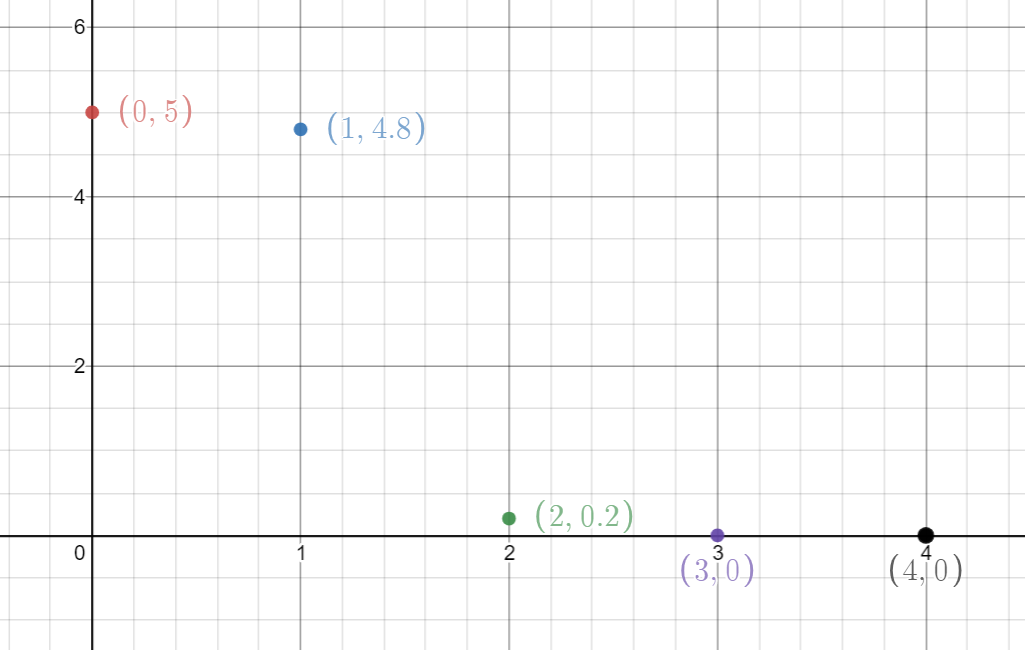
The most simple interpolation technique is to define a piecewise linear function in-between each pair of data points (linear interpolation). Then we can approximate this continuous function for any value of \(x\) by evaluating the appropriate linear function:

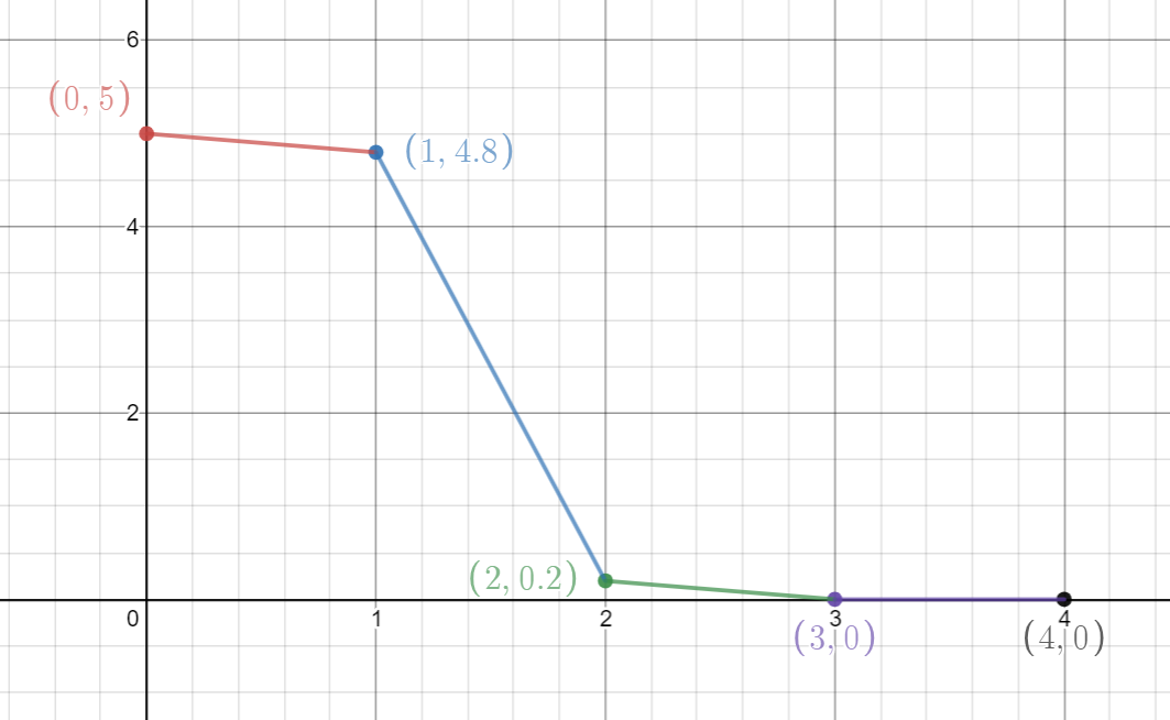
Linear Interpolation is simple to implement and fast to evaluate, and is regularly a suitable choice in computer graphics. But the approximation does not yield a smooth function.

This property can sometimes be undesirable - for instance, imagine a ball moving at constant velocity along our approximated function. The discontinuous derivative would lead to the ball changing direction instantaneously at each data point, rather than smoothly changing direction.

To rectify this, one can choose a higher-order polynomial in-between each pair of data points, and we can author the gradients of this polynomial to ensure the overall approximated function is both continuous, and has a continuous derivative. One common choice here is to use a cubic hermite polynomial - a cubic polynomial that is expressed in terms of its end-point values and gradients:

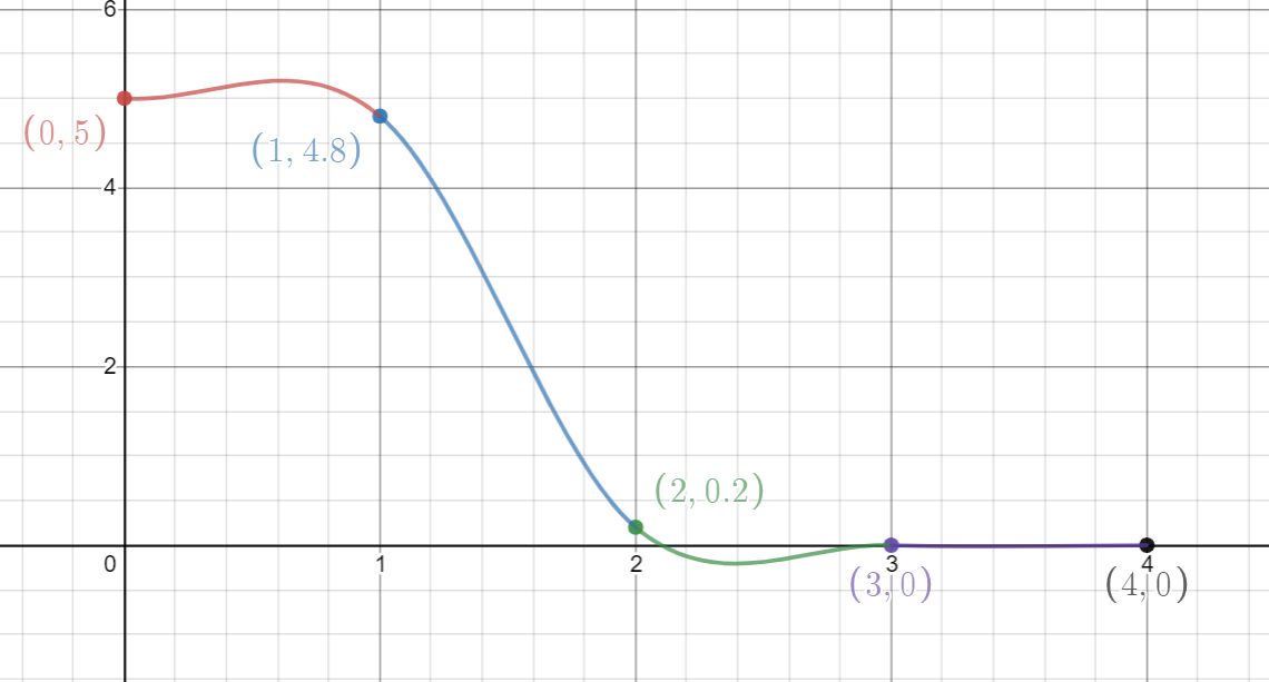
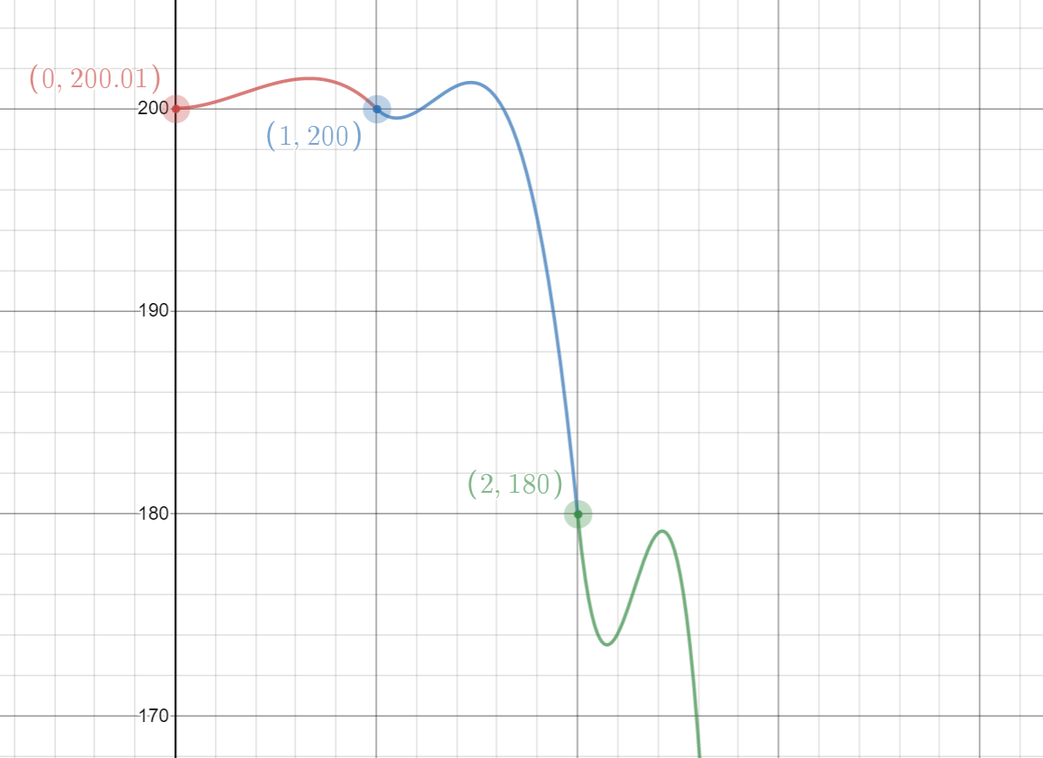
This results in a much smoother approximation - the overall approximation is both continuous and has a continuous first derivative, which fixes the abrupt change in gradient in the linearly interpolated case. But this also introduces a problem - the curve now overshoots outside the bounds of our data point values:

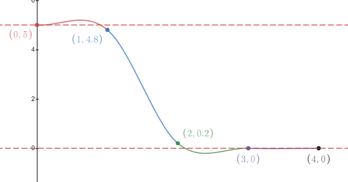
Why Is This A Problem?

In computer graphics, this overshoot can lead to values that fall outside the expected range of values for the domain we are working in. For instance, suppose the above curve represents volume density. Our approximation takes us below zero which in real-life, would represent negative density. There is no correponding real-life scenario where this would ever happen. So, if we were rendering this volume, this error might lead to visual artefacts (for instance, areas of missing volume). If we were performing a physical simulation with this volume (for instance, if this volume represented fluid pressure), this sort of error could introduce divergence into the resultant simulation, and therefore loss of volume, and accumulation of this error over time could eventually lead to a broken simulation.

How Bad Can It Get?

The following graph shows just how bad this can get. Here, we’re interpolating between the following points: (0, 200.01), (1, 200), (2, 180), (3, 0), (4, -800).

These have been deliberately authored to cause overshoots at each segment of our curve, but the values are clearly strictly decreasing in y, and yet the resultant curve is not:

Goal: Preserving Monotonicity

Another way of describing this problem, is to say that our approximation no longer preserves the monotonicity of our data points. Our data points are decreasing, and yet the approximation is not monotonic since the wiggles caused by overshoot lead to areas of the curve that are also increasing. This too could also be a problem - for instance, in cases where we are working with some underlying assumption that the curve is always decreasing.

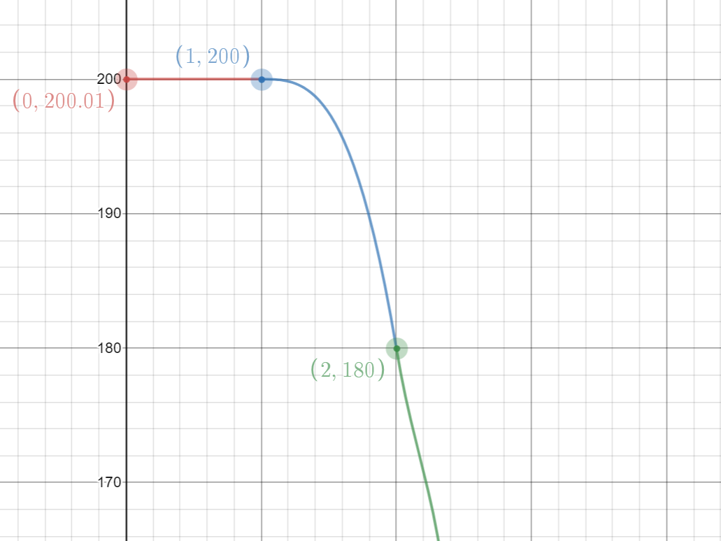
To jump straight to the results of this post, the following image shows the same data points but with monotone cubic interpolation instead. As we can see, the curve is still smooth, but also stays within the bounds of the data points:

The Cubic Hermite Polynomial

The cubic hermite polynomial is defined as follows:

where:

• \(t\) is the interpolation parameter, with \(0 \le t \le 1\)
• \(p_i\) is the curve value at \(t=0\), taken directly from the data point at this location
• \(p_{i+1}\) is the curve value at \(t=1\), taken directly from the data point at this location
• \(\delta_i\) is the desired gradient at \(t=0\)
• \(\delta_{i+1}\) is the desired gradient at \(t=1\)

The gradients \(\delta_i\) and \(\delta_{i+1}\) are chosen to be continuous with the neighbouring cubic polynomials, by using two-sided differences in the interior of the curve, and one-sided differences on the first and last data points.

Conditions for Monotonicity

The paper Monotone Piecewise Cubic Interpolation by Fritsch and Carlson presents the various conditions that need to be satisfied in order to guarantee monotonicity for a cubic hermite polynomial, along with a procedure for ensuring that a set of piecewise cubic hermite polynomials preserve monotonicity of the data points.

In order to gain a better understanding of these conditions, I studied the paper and explore these graphically in this section.

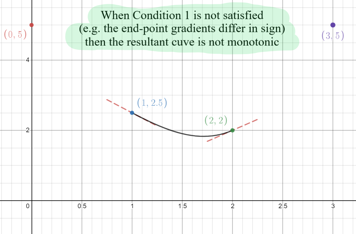
Condition 1: Sign of Data Point Gradients Must Be Equal To Sign of Secant Gradient

We are considering a single cubic polynomial here (e.g. for a single pair of data points). Let \(\Delta_i\) be the gradient of the secant line connecting the two data points, with \(\Delta_i = p_{i+1} - p_i\). In order to preserve the monoticity of the data points, the sign of this gradient dictates whether we would like this cubic to be increasing or decreasing, and since we want this cubic to be monotonic, the sign of the gradient at all points along this curve must be consistent (and match the sign of \(\Delta_i\)).

If either of the end-points have gradients that differ in sign to that of \(\Delta_i\), then we know that the curve does not preserve the monotonicity of the data points. For instance, in the image below, the data points are decreasing and so we would like a negative gradient at all points on the polynomial, and yet the gradient of the end-point is positive:

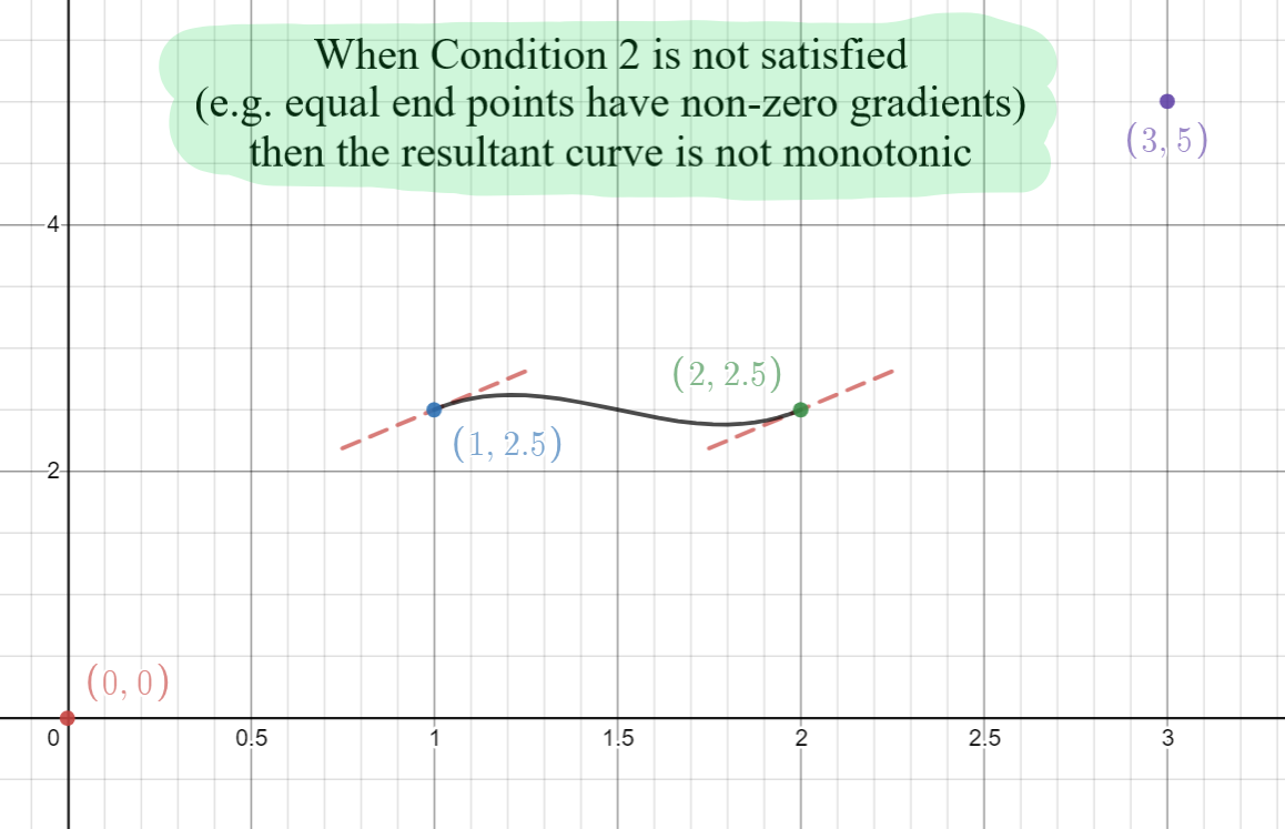
Condition 2: An Equal Pair Of Data Point Values Must Have Zero Data Point Gradients

If both data points have exactly the same value, then the gradient of the secant line connecting these two points will be exactly zero (e.g. \(\Delta_i = 0\)). We would expect to see a straight horizontal line between the two data points in this case, and so the end-point gradients must equal zero. If either of the gradients are not zero then the curve between these two points will not be monotonic:

Condition 3: When \(\alpha_i + \beta_i - 2 \le 0\), Condition 1 Ensures Monotonicity

Lets now suppose that the above two conditions are true, e.g:

At this point, it is convenient to rearrange the cubic hermite equation in terms of its parameter \(t\), and substituting \(\Delta_i\) we have:

and the first derivative of this function is as follows:

The paper shows that there are two general cases that we need to consider here:

• When \(\delta_i + \delta_{i+1} - 2 \Delta_i = 0\)

  • \(g(t)\) simplifies to a quadratic and \(g'(t)\) becomes linear and is therefore either constant, increasing, or decreasing. The condition \(\text{sign}(\Delta_i) = \text{sign}(\delta_i) = \text{sign}(\delta_{i+1})\) already prevents \(g'(t)\) from changing signs. So this condition alone is sufficient to ensure that the curve remains monotonic

• When \(\delta_i + \delta_{i+1} - 2 \Delta_i \neq 0\)

  • In this case, the derivative \(g'(t)\) is a quadratic and so \(g'(t) = 0\) has up to two unique solutions in \(t\). To preserve monotonicity we need to ensure that there are no such solutions in \(t \in \left[ 0, 1 \right]\).

    There are two orthogonal properties of \(g(t)\) and \(g'(t)\) that are explored in this case:

    • Whether the gradient of the secant line between end-points \(\Delta_i\) is positive or negative
    • Whether the derivative \(g'(t)\) is concave-up or concave-down

    Each of these combinations is illustrated below, with the curve itself drawn in solid-red, and its first derivative drawn in dashed-blue:

    

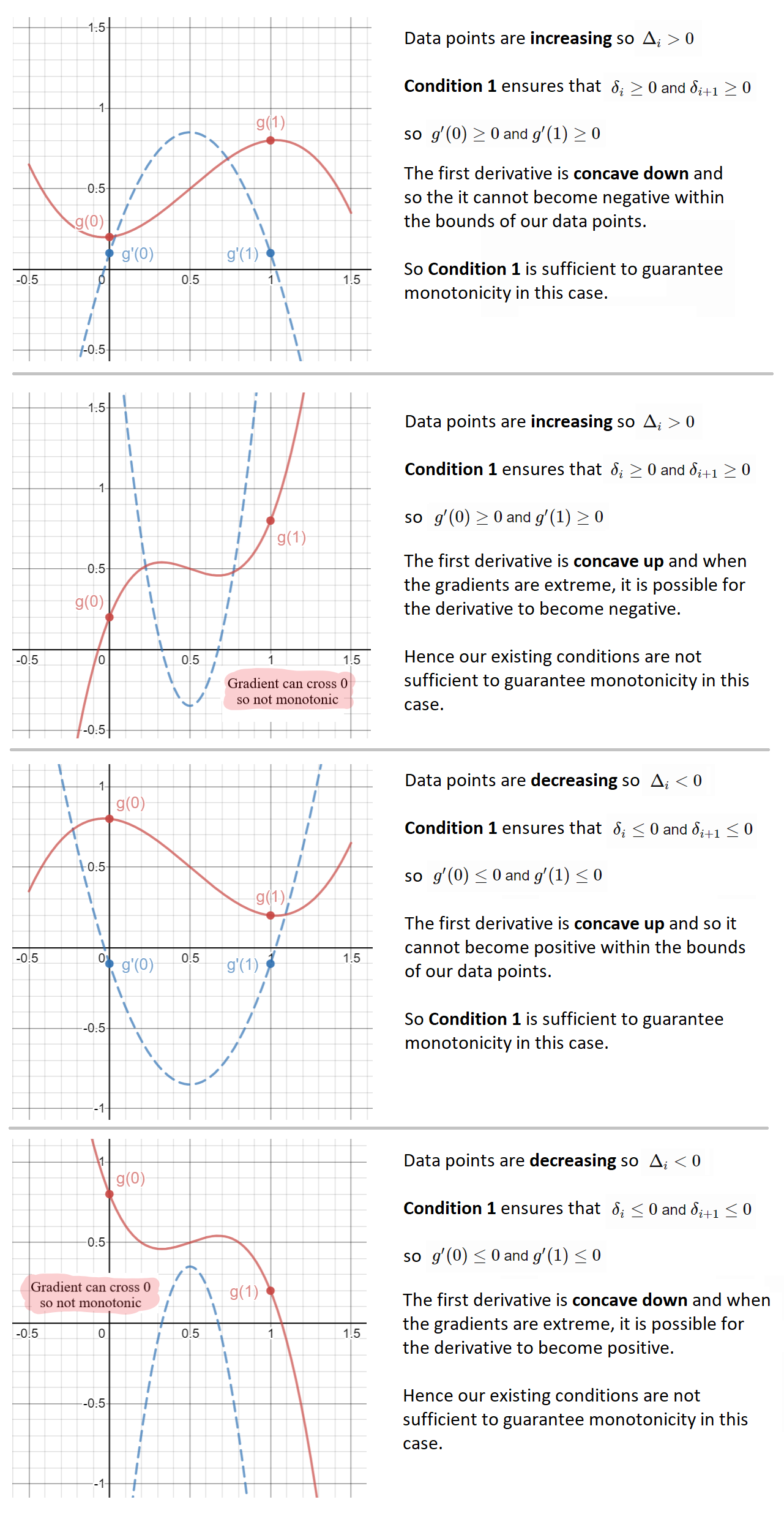
    So, for two of these four cases, monotonicity is already preserved by condition 1. For the remaining cases, it can be seen above that large gradient values can cause the first derivative to change signs and hence no longer preserve monotonicity.

    To summarise:

    • If \(\delta_i + \delta_{i+1} - 2 \Delta_i > 0\) and \(\Delta_i < 0\), monotonicity is preserved
    • If \(\delta_i + \delta_{i+1} - 2 \Delta_i < 0\) and \(\Delta_i > 0\), monotonicity is preserved

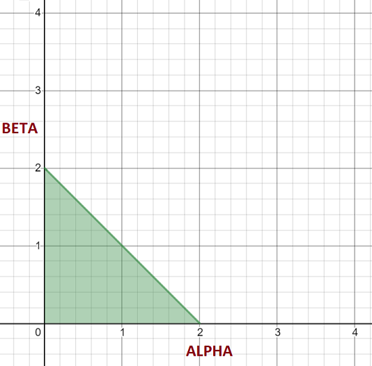
    The paper summarises both of these conditions elegently in a single constraint by dividing throughout by \(\Delta_i\) and letting \(\alpha_i = \delta_i / \Delta_i\) and \(\beta_i = \delta_{i+1} / \Delta_i\):

    • If \(\alpha_i + \beta_i - 2 \le 0\), condition 1 ensures monotonicity is preserved

    This is nicely presented in the paper by plotting this constraint on a graph, where \(\alpha\) and \(\beta\) are the \(x\) and \(y\) axes respectively. If we have a cubic polynomial whose \(\alpha_i\) and \(\beta_i\) values are inside the green region, then the cubic polynomial is monotonic:

    

Condition 4: When \(\alpha_i + \beta_i - 2 > 0\), Gradients May Need To Be Restricted

Of the remaining cubic polynomials where \(\alpha_i + \beta_i - 2 > 0\), we have seen in the diagrams above that if the end-point gradients happen to be extreme enough, the first derivative may change sign and yield a curve that is not monotonic.

Of the remaining cases, this will happen when the first derivative has a local extremum that strays beyond \(g'(t) = 0\) when \(0 \le t \le 1\).

To determine when this happens, we can examine the second derivative:

Putting \(g''(t) = 0\) and dividing throughout by \(\Delta_i\) (allowing us to substitute \(\alpha\) and \(\beta\)) we can find the value of \(t\) for which this local extremum occurs:

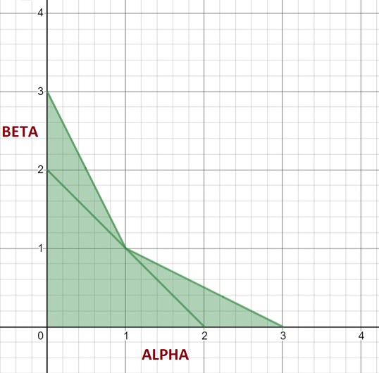
• If this local extremum is not in the range \((0,1)\), then for all points on the curve within this range, the first derivative will be monotonic and since condition 1 already ensures that the first derivative at both end-points has a consistent sign, the first derivative has no opportunity to change signs and so the curve itself is monotonic in this case. Since \(\alpha + \beta - 2 > 0\), this case happens when either of the following are true:

  \[2 \alpha + \beta - 3 \le 0 \\ \alpha + 2 \beta - 3 \le 0\]

  We can see this clearly by plotting these additional regions on our monotonicity graph:

  

• If this local extremum is inside the range \((0,1)\), then we want to ensure it doesn’t change signs. That is, the sign of the local extremum must be consistent with the sign of \(\Delta_i\) (because if the first derivative changes sign, our curve is not monotonic).

  The value of the first derivative at this extremum is as follows:

  \[g'(\hat{t}) = \Delta_i \left\{ \alpha - {1 \over 3} \left[ \frac{\left( 2 \alpha + \beta - 3 \right)^2}{\alpha + \beta - 2} \right] \right\}\]

  and we want:

  \[\text{sign}(g'(\hat{t})) = \text{sign}(\Delta_i)\]

  which means that the following condition must be true for our curve to be monotonic:

  \[\alpha - {1 \over 3} \left[ \frac{\left( 2 \alpha + \beta - 3 \right)^2}{\alpha + \beta - 2} \right] \ge 0\]

  Adding this constraint to our monotonicity graph gives us a complete region for monotonicity - any cubic polynomials whose \(\alpha_i\) and \(\beta_i\) values fall outside this range are not monotonic:

  

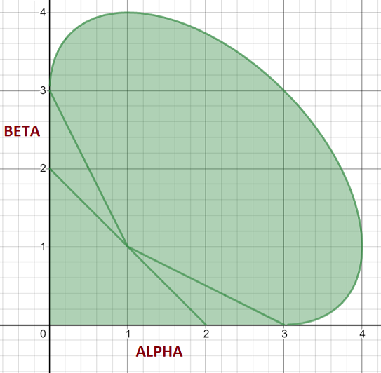
  The paper shows that we can make any cubic hermite polynomial monotonic by restricting the values of \(\alpha_i\) and \(\beta_i\) (and hence \(\delta_i\) and \(\delta_{i+1}\)) to ensure they are inside this safe region.

Sampling vs Gradient Conditioning

An algorithm for conditioning the gradients of a set of data points to preserve monotonicity is presented in the Fritsch-Carlson paper. An implementation of this algorithm is outlined with some example code in the Wikipedia page Monotone Cubic Interpolation. In both cases, the algorithm is based on the assumption that you are storing these gradients and able to modify them.

In some circumstances this might not be possible. For instance, in the domain of volume rendering for feature-film quality visual effects, the data that you wish to interpolate can be very dense and consume gigabytes of memory. Storing these gradients (rather than computing them on-the-fly) would be both time consuming and have a large impact on memory footprint. This is made worse by the fact that within this domain, the data is 3-dimensional, and the desired interpolation scheme is actually tri-cubic, where interpolated data points in one axis are then used as data points for the next axis, and so on.

In this case it is necessary to sample a fixed number of data points and then use these data points to calculate monotonic gradients that can be evaluated immediately.

Do These Samplers Really Preserve Monoticity?

The motivation for studying this paper and writing this post in the first place, was as result of encountering existing literature and implementation in the computer graphics community that claim to preserve monotonicity for piecewise cubic interpolation, and yet do not handle all of these conditions.

Armed with our knowledge about the various mathematical conditions that need to be satisfied in order to guarantee monotonicity, we can take a look at some of these sources, and critically evaluate them. I must stress that the goal of doing this is to illustrate with real world examples, that it can be easy to encounter an implementation in the public domain that doesn’t satisfy these conditions, and that it can also be easy to underestimate the conditions that need to be satisfied in order to guarantee monotonicity - I am certainly not judging the original authors in any way here.

I first encountered this problem when reading about monotone cubic interpolation in the excellent Production Volume Rendering book. The book presents a monotone cubic sampler whose implementation is also widely used in the open source community via the Field3D library:

// From: https://github.com/imageworks/Field3D/blob/master/export/FieldInterp.h
template<class T>
T monotonicCubicInterpolant(const T &f1, const T &f2, const T &f3, const T &f4, 
                            double t)
{
  T d_k = T(.5) * (f3 - f1);
  T d_k1 = T(.5) * (f4 - f2);
  T delta_k = f3 - f2;

  // EDIT: This condition isn't sufficient to guarantee monotonicity
  if (delta_k == static_cast<T>(0)) {
    d_k = static_cast<T>(0);
    d_k1 = static_cast<T>(0);
  }

  T a0 = f2;
  T a1 = d_k;
  T a2 = (T(3) * delta_k) - (T(2) * d_k) - d_k1;
  T a3 = d_k + d_k1 - (T(2) * delta_k);

  T t1 = t;
  T t2 = t1 * t1;
  T t3 = t2 * t1;

  return a3 * t3 + a2 * t2 + a1 * t1 + a0;
}

• The implementation satisfies Condition 2 discussed above (e.g. if both data points are equal, then the polynomial should be a straight line, with gradients both equal to 0)
• But it satisfies this condition weakly due to floating-point rounding error (only if delta_k exactly equals zero)
• The other conditions are not satisfied. It is therefore possible to feed this function a set of monotonic data points that do not result in a monotonic curve

This problem is acknowledged in the GitHub issue “Fix monotonic cubic interpolation” and the proposed solution is to change the monotonicity test to the following:

if (delta_k == static_cast<T>(0) || (sign(d_k) != sign(delta_k) || sign(d_k1) != sign(delta_k))) {
    d_k = static_cast<T>(0);
    d_k1 = static_cast<T>(0);
}

I believe the source of this statement is the paper Visual Simulation of Smoke by Fedkiw et al, which is cited by the Production Volume Rendering book as being the inspiration behind this scheme. This paper states the following conditions as being necessary to guarantee monotonicity:

• Whilst these conditions are indeed necessary (both Condition 1 and Condition 2 are satisfied), the paper by Fritsch and Carlson show that these are not the only conditions that need to be satisfied in order to guarantee monotonicity
• Specifically, Condition 4 shows that even if the above conditions are true, if the gradients happen to be extreme enough, the first derivative can still cross \(g'(t) = 0\), which by definition
• So likewise, it would also be possible to feed this modified function a set of monotonic data points that do not result in a monotonic curve (example)

Making A Cubic Hermite Curve Monotonic

The paper shows that there are a number of strategies that can be employed to modify your curve gradients such that they reside inside the monotonicity region. The technique suggested in the paper is to first compute \(\alpha\) and \(\beta\), and calculate new values \(\alpha^*\) and \(\beta^*\) such that these new values are within a circle of radius 3 (which is fully encapsulated inside the monotonicity region).

• First, check whether your \(\alpha_i\) and \(\beta_i\) values fall outside the circle of radius 3:

  \[\alpha_i^2 + \beta_i^2 > 9\]

• If they do, calculate a scaling factor \(\tau\) that puts these values back onto the circle of radius 3:

  \[\begin{align} \tau_i &= {3 \over \sqrt{\alpha_i^2 + \beta_i^2}} \\ \alpha_i^* &= \tau_i \cdot \alpha_i \\ \beta_i^* &= \tau_i \cdot \beta_i \end{align}\]

• Then our new gradients can be calculated as follows:

  \[\begin{align} \delta_i = \alpha_i^* \Delta_i &= \tau_i \alpha_i \Delta_i \\ \delta_{i+1} = \beta_i^* \Delta_i &= \tau_i \beta_i \Delta_i \end{align}\]

Floating Point Rounding Error Can Also Break Monotonicity

One of the advantages of preserving monotonicity is that the resultant interpolated values are guaranteed to remain inside the range defined by the data points. In some cases, this is essential - for instance, if you are working with values that should never fall below zero.

Whilst mathematically, the steps detailed above ensures this, when it comes to implementation, the rounding error introduced by floating point arithmetic can also cause the resultant interpolated values to stray out of expected bounds.

We can take advantage of the monotonicity property, by noting that a monotonic function \(f : [a,b] \rightarrow \mathbb{R}\) defined on \([a, b]\) is bounded above by \(\max\{f(a), f(b)\}\) and bounded below by \(\min\{f(a), f(b)\}\). We can therefore clamp the resultant interpolated value between the minimum of the end-point values, and the maximum end-point values as an additional guard to prevent rounding error from breaking the monotonicity of our interpolated values.

Implementing a Fritsch-Carlson Sampler

When you are working with multiple data points, with a cubic hermite curve joining each successive pair of data points, consistent end-point gradients must be chosen to maintain C1 continuity overall.

Recall that we are interested in a sampling approach here, where data points are directly sampled in order to calculate the desired gradients on-the-fly (e.g. no storage and pre-conditioning of these gradients). In order to maintain C1-continuity, it is therefore necessary to sample the neighbouring cubic hermite curves as well, and have a rule for choosing consistent end-point gradients. Since the technique above results in a reduction of gradient magnitudes, an approach we can take here is to consider the cubic hermite curve to the left and the right of each end-point, and if we happen to modify gradient values, ensure we pick the gradient values closest to zero.

This gives rise to the following cubic hermite sampler, which also guarantees monotonicity using the Fritsch-Carlson technique (in Rust):

/// Monotone cubic interpolation of values y0 and y1 using x as the interpolation
/// parameter (assumed to be [0..1]). A modification of hermite cubic interpolation
/// that prevents overshoots (preserves monoticity). In order to both maintain
/// monotonicity and C1 continuity, two neighbouring samples to the left of y0 and
/// the right of y1 are also necessary
pub fn interpolate_cubic_monotonic_fritsch_carlson(
    x: f32,
    y_minus_2: f32,
    y_minus_1: f32,
    y0: f32,
    y1: f32,
    y2: f32,
    y3: f32,
) -> f32 {
    // Calculate secant line gradients for each successive pair of data points
    let s_minus_2 = y_minus_1 - y_minus_2;
    let s_minus_1 = y0 - y_minus_1;
    let s_0 = y1 - y0;
    let s_1 = y2 - y1;
    let s_2 = y3 - y2;

    // Use central differences to calculate initial gradients at y_minus_1, y0, y1, y2
    // respectively...
    let mut m_minus_1 = (s_minus_2 + s_minus_1) * 0.5;
    let mut m_0_left = (s_minus_1 + s_0) * 0.5;
    let mut m_1_left = (s_0 + s_1) * 0.5;
    let mut m_2 = (s_1 + s_2) * 0.5;

    // ... Note that in order to maintain C1 continuity, we calculate gradients that
    // preserve monotonicity for the curves to the left and right of each end point,
    // and then pick the gradients with the smallest magnitude, hence why there is a
    // 'left' and 'right' variable for each end-point gradient here (initially,
    // they are the same).
    let mut m_0_right = m_0_left;
    let mut m_1_right = m_1_left;

    // If the central curve (joining y0 and y1) is neither increasing or decreasing, we
    // should have a horizontal line, so immediately set gradients to zero here.
    if relative_eq!(y0, y1) {
        m_0_right = 0.0;
        m_1_left = 0.0;
    } else {
        // Now examine the curve to the left of y0 and the right of y1. If either should
        // be horizontal lines, then immediately set the corresponding end-point gradients
        // to zero here.
        if relative_eq!(y_minus_1, y0) {
            m_0_left = 0.0;
        }
        if relative_eq!(y1, y2) {
            m_1_right = 0.0;
        }

        // If secant line gradients either side of each end point have opposite signs,
        // must constrain the gradients to zero.
        if s_minus_2 < 0.0 && s_minus_1 >= 0.0 || s_minus_2 > 0.0 && s_minus_1 <= 0.0 {
            m_minus_1 = 0.0;
        }

        if s_minus_1 < 0.0 && s_0 >= 0.0 || s_minus_1 > 0.0 && s_0 <= 0.0 {
            m_0_left = 0.0;
            m_0_right = 0.0;
        }
        if s_0 < 0.0 && s_1 >= 0.0 || s_0 > 0.0 && s_1 <= 0.0 {
            m_1_left = 0.0;
            m_1_right = 0.0;
        }

        if s_1 < 0.0 && s_2 >= 0.0 || s_1 > 0.0 && s_2 <= 0.0 {
            m_2 = 0.0;
        }

        // Calculate alpha and beta values for the left, centre, and right curves.
        let (alpha_left, beta_left) = if s_minus_1 != 0.0 {
            (m_minus_1 / s_minus_1, m_0_left / s_minus_1)
        } else {
            (0.0, 0.0)
        };

        let (alpha_cent, beta_cent) = if s_0 != 0.0 {
            (m_0_right / s_0, m_1_left / s_0)
        } else {
            (0.0, 0.0)
        };

        let (alpha_right, beta_right) = if s_1 != 0.0 {
            (m_1_right / s_1, m_2 / s_1)
        } else {
            (0.0, 0.0)
        };

        // Calculate the discriminant on the left, centre, and right curves.
        let disc_left = (alpha_left * alpha_left) + (beta_left * beta_left);
        let disc_cent = (alpha_cent * alpha_cent) + (beta_cent * beta_cent);
        let disc_right = (alpha_right * alpha_right) + (beta_right * beta_right);

        // Calcuate the constrained end-point gradients on the left, centre,
        // and right curves.
        if disc_left > 9.0 {
            m_0_left = 3.0 / disc_left.sqrt() * beta_left * s_minus_1;
        }

        if disc_cent > 9.0 {
            m_0_right = 3.0 / disc_cent.sqrt() * alpha_cent * s_0;
            m_1_left = 3.0 / disc_cent.sqrt() * beta_cent * s_0;
        }

        if disc_right > 9.0 {
            m_1_right = 3.0 / disc_right.sqrt() * alpha_right * s_1;
        }
    }

    // Choose the gradients with the smallest magnitude.
    let m_0 = if m_0_left.abs() < m_0_right.abs() {
        m_0_left
    } else {
        m_0_right
    };
    let m_1 = if m_1_left.abs() < m_1_right.abs() {
        m_1_left
    } else {
        m_1_right
    };

    // Evaluate the cubic hermite spline
    let result =
        (((((m_0 + m_1 - 2.0 * s_0) * x) + (3.0 * s_0 - 2.0 * m_0 - m_1)) * x) + m_0) * x + y0;

    // The values at the end points (y0 and y1) define an interval that the curve passes
    // through. Since the curve between the end-points is now monotonic, all interpolated
    // values between these end points should be inside this interval. However, floating
    // point rounding error can still lead to values slightly outside this range.
    // Guard against this by clamping the interpolated result to this interval...
    let min = y0.min(y1);
    let max = y0.max(y1);
    result.min(max).max(min)
}

The advantage of this function is that it yields visually pleasing results that preserve monotonicity and C1-continuity. But in particular, maintaining C1 continuity comes at the cost of having to perform 6 samples and a lot of arithmetic. It would be nice if we could find a cheaper solution here…

A More Efficient Monotone-Cubic Sampler

The approach taken above is based on the observation that a circle of radius \(3\) is entirely encapulated by the monotonicity region. But this is one of a handful of techniques that you could try. For instance, observe that \((0,0)\) is inside the monotonicity region, and so setting \(\alpha = \beta = 0\) would guarantee monotonicity (this would lead to gradients of \(0\) everywhere, which would not look very visually appealing).

Alternatively, notice that the cube with corners defined at \((0, 0)\) and \((3, 3)\) is also fully encapsulated by the monotonicity region. So constraining \(\alpha_i \le 3\) and \(\beta_i \le 3\) is also sufficient. This alternative is cited in the Fritsch-Carlson paper, and is also the basis of the paper Non-Overshooting Hermite Cubic Splines for Keyframe Interpolation by Heckbert.

To constrain a curve such that its \(\alpha_i\) and \(\beta_i\) values are inside this cube:

• If \(\alpha_i > 3\) we set \(\alpha_i = 3\) resulting in a new gradient of \(\delta_i = 3 \Delta_i\)
• If \(\beta_i > 3\) we set \(\beta_i = 3\) resulting in a new gradient of \(\delta_{i+1} = 3 \Delta_i\)

When working with a set of piecewise cubic hermite curves, care must still be taken to evaluate this constraint on the left and right of each end-point, but the advantage of the above constraints is that they only depend on the secant values, which can be computed with just four samples.

This gives rise to the following cubic hermite sampler, which still guarantees monotonicity and C1-continuity but requires less samples and less arithmetic (again, in Rust):

/// Monotone cubic interpolation of values y0 and y1 using x as the interpolation
/// parameter (assumed to be [0..1]). A modification of hermite cubic interpolation
/// that prevents overshoots (preserves monoticity). In order to both maintain
/// monotonicity and C1 continuity, two neighbouring samples to the left of y0 and
/// the right of y1 are also necessary
pub fn interpolate_cubic_monotonic_heckbert(
    x: f32,
    y_minus_1: f32,
    y0: f32,
    y1: f32,
    y2: f32
) -> f32 {
    // Calculate secant line gradients for each successive pair of data points
    let s_minus_1 = y0 - y_minus_1;
    let s_0 = y1 - y0;
    let s_1 = y2 - y1;

    // Use central differences to calculate initial gradients at the end-points
    let mut m_0 = (s_minus_1 + s_0) * 0.5;
    let mut m_1 = (s_0 + s_1) * 0.5;

    // If the central curve (joining y0 and y1) is neither increasing or decreasing, we
    // should have a horizontal line, so immediately set gradients to zero here.
    if relative_eq!(y0, y1) {
        m_0 = 0.0;
        m_1 = 0.0;
    }
    else {
        // If the curve to the left is horizontal, or the sign of the secants on either side
        // of the end-point are different, set the gradient to zero...
        if relative_eq!(y_minus_1, y0) || s_minus_1 < 0.0 && s_0 >= 0.0 || s_minus_1 > 0.0 && s_0 <= 0.0 {
            m_0 = 0.0;
        }
        // ... otherwise, ensure the magnitude of the gradient is constrained to 3 times the
        // left secant, and 3 times the right secant (whatever is smaller)
        else {
            m_0 *= (3.0 * s_minus_1 / m_0).min(3.0 * s_0 / m_0).min(1.0);
        }

        // If the curve to the right is horizontal, or the sign of the secants on either side
        // of the end-point are different, set the gradient to zero...
        if relative_eq!(y1, y2) || s_0 < 0.0 && s_1 >= 0.0 || s_0 > 0.0 && s_1 <= 0.0 {
            m_1 = 0.0;
        }
        // ... otherwise, ensure the magnitude of the gradient is constrained to 3 times the
        // left secant, and 3 times the right secant (whatever is smaller)
        else {
            m_1 *= (3.0 * s_0 / m_1).min(3.0 * s_1 / m_1).min(1.0);
        }
    }

    // Evaluate the cubic hermite spline
    let result =
        (((((m_0 + m_1 - 2.0 * s_0) * x) + (3.0 * s_0 - 2.0 * m_0 - m_1)) * x) + m_0) * x + y0;

    // The values at the end points (y0 and y1) define an interval that the curve passes
    // through. Since the curve between the end-points is now monotonic, all interpolated
    // values between these end points should be inside this interval. However, floating
    // point rounding error can still lead to values slightly outside this range.
    // Guard against this by clamping the interpolated result to this interval...
    let min = y0.min(y1);
    let max = y0.max(y1);
    result.min(max).max(min)
}

Conclusion

To conclude, it is often desirable to maintain the monotonicity of data points when interpolating between them, and this is not guaranteed when using cubic hermite polynomials. The Fritsch-Carlson paper presents each of the conditions that must be satisfied in order to preserve monotonicity, and by looking at a handful of implementations in the public domain that do not handle all of these cases, I’ve hopefully shown that it can be easy to overlook these. We’ve walked through each of these conditions visually, and then provided two implementations that handle piecewise cubic hermite polynomials. In particular, the approach we have taken here is a sampling approach, where gradients are not stored and pre-conditioned prior to interpolation.

References

Fedkiw, R., Stam, J. and Jensen, H.W, “Visual Simulation of Smoke”, SIGGRAPH 2001, 23-30 (2001).

Field3D - https://github.com/imageworks/Field3D

Fritsch, F. N., and R. E. Carlson. “Monotone Piecewise Cubic Interpolation.” SIAM Journal on Numerical Analysis, vol. 17, no. 2, 1980, pp. 238–246.

Heckbert, P. “Non-Overshooting Hermite Cubic Splines for Keyframe Interpolation”.

Wikipedia contributors, “Monotone cubic interpolation,” Wikipedia, The Free Encyclopedia, https://en.wikipedia.org/w/index.php?title=Monotone_cubic_interpolation&oldid=950478742 (accessed December 16, 2020).

Wrenninge, Magnus. (2012). Production volume rendering: Design and implementation. 10.1201/b12698.