Computing Coordinate Frames on a Spline with Minimal Torsion
Over the past few days I have been experimenting with some algorithms for generating procedural tree meshes. While there are many steps involved, a significant step in the process is to generate a mesh for each branch of the tree.
A branch is typically represented as a spline. One can generate a mesh by incrementally sliding a disc (or any cross-sectional curve) along the spline. At each position, you orient the disk and then join the disk’s edge vertices to the vertices of the disk at the previous position. This is often referred to as a “generalised cylinder”.
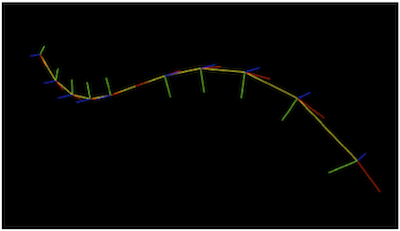
In order to orient the disk at each position, you need to generate a coordinate frame for each position. One possible technique is to compute the Frenet Frame by analytically evaluating the curve function, its first derivative, and its second derivative, and then using the Frenet equations to find the tangent, primary normal, and binormal vectors. This is shown in the following image, where the red vectors represent the tangents, green vectors represent the primary normals, and blue vectors represent the binormals.

As shown in the above image, analytically computing the Frenet Frame at regular intervals along the spline introduces some problems:
-
The primary normal is computed using the second derivative, which is zero at inflection points. This means that the primary normal and binormal is undefined at these locations (notice in the above image, the coordinate frame at the inflection point is missing a normal and binormal)
-
The primary normal is defined to point in the direction of curvature. At inflection points, the direction of curvature changes, and this results in the normal being inverted
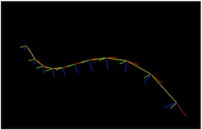
If you can live without your normal pointing in the direction of curvature (I certainly can), a common solution to this problem is to define a world up-axis, and then compute a normal by evaluating the cross product of this world-up axis with the tangent vector. The cross product of the resultant normal and the tangent vector can then be evaluated to find the binormal. Applying this approach to the scenario as shown in the previous image is shown below:

The above image looks a lot better (the normal and binormal has been fixed at the inflection point, and the inflection point hasn’t affected the orientation of the normals). But what if your tangent happens to be pointing in the same direction as your chosen world-up axis? This scenario is shown in the image below:

As the image above shows, this also leads to undesired rotations in the coordinate frames (shown at the minimum and maximum points of the curve in the above image).
The twisting rotation about the tangent vector is often described as torsion. We need a sliding coordinate frame that minimises torsion. Jules Bloomenthal has a good article on the subject, published in the first Graphics Gems book (and available in PDF form here.
The basic idea is as follows: instead of analytically computing a coordinate frame at each point, we compute an initial coordinate frame at the beginning of the curve and then propagate this coordinate frame along the curve in small increments. At each step, we rotate the coordinate frame into place.
Given the previous coordinate frame T, N, B, one can compute the next coordinate frame T’ N’ and B’ as follows:
- Compute T’ analytically, by evaluating the first derivative of the curve
- Compute the axis of rotation from T to T’ by taking the cross product of T and T’, and then normalizing
- Compute the angle of rotation by computing the angle between T and T’
- Rotate N using the axis and angle computed above to find N’
- Compute the cross product of T’ and N’ to find B’
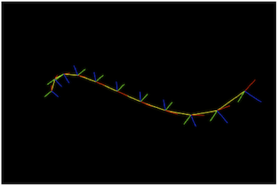
This is a really useful technique because it is not affected by points of inflection or curves whose control points are arranged to yield a straight line. It also doesn’t depend on a particular axis (such as an up-axis), and is therefore not prone to undesired torsion when the tangent is aligned with this particular axis.